Example 6: rising bubble in an imposed flow (advection + AMR)

Files

• 2D test file: main.cpp
• 3D test file: main.cpp
• Velocity field: coefficient.json in each test directory

Statement of the problem

This test is adapted from a rising bubble problem of C. Introïni's PhD thesis¹. It validates the advection integrators (SplitAdvection, AdvectionBoundaryCH) coupled with the Cahn-Hilliard equations, with adaptive mesh refinement.

A bubble is transported by an imposed velocity field $\mathbf{v}$ (no Navier-Stokes equations are solved):

$$\begin{align} \frac{\partial \phi}{\partial t}&= \nabla\cdot\left(M\nabla \mu\right) - \nabla\cdot\left(\phi\,\mathbf{v}\right) \text{ in }\Omega \\[6pt] \mu &= \omega W'(\phi) - \lambda \Delta \phi \text{ in }\Omega \end{align}$$

where $\phi$ is the phase indicator ($\phi=0$ in the bubble, $\phi=1$ in the surrounding matrix), $\mu$ the generalized chemical potential and $W$ the double-well potential:

$$\begin{align} W(\phi)&=\phi^2(1-\phi)^2, \qquad \lambda=\frac{3}{2}\sigma\epsilon, \qquad \omega=\frac{12\sigma}{\epsilon} \end{align}$$

The 2D domain $\Omega$ is the rectangle $[0,R]\times[0,H]$ with $R=5r_b$ and $H=8r_b$, where $r_b$ is the bubble radius. The imposed velocity is a Poiseuille-like profile, vanishing on the lateral walls and divergence-free:

$$\mathbf{v} = v_{max}\left[1-\left(\frac{x-R/2}{R/2}\right)^2\right]\mathbf{e}_y$$

In 3D, the domain is $[0,R]\times[0,H]\times[0,R]$ ($y$ is the vertical direction) and the profile is parabolic in both transverse directions:

$$\mathbf{v} = v_{max}\left[1-\left(\frac{x-R/2}{R/2}\right)^2\right]\left[1-\left(\frac{z-R/2}{R/2}\right)^2\right]\mathbf{e}_y$$

Initial condition

The bubble is centred at $(R/2, 3r_b)$ in 2D ($(R/2, 3r_b, R/2)$ in 3D):

$$\phi = \frac{1}{2} + \frac{1}{2}\tanh\left(\frac{2\left(r - r_b\right)}{\epsilon}\right), \qquad \mu = 0$$

where $r$ is the distance to the bubble centre. $\mu=0$ corresponds to the equilibrium of the planar tanh profile ($\omega W'(\phi)=\lambda\phi''$ since $\lambda/\omega=\epsilon^2/8$).

Parameters used for the test

The physical data are those of the rising bubble problem with $Bo=10$ and $Mo=10^{-2}$, the radius being deduced from the Bond number: $r_b = 0.5\sqrt{\sigma Bo/\left(g(\rho_2-\rho_1)\right)}$.

Name	Description	Symbol	Value
sigma	interfacial energy	$\sigma$	$7\times 10^{-2}$ J.m$^{-2}$
rho1, rho2	gas and liquid densities	$\rho_1, \rho_2$	$1$, $10^3$ kg.m$^{-3}$
bond	Bond number	$Bo$	$10$
rb	bubble radius	$r_b$	$4.226\times 10^{-3}$ m
epsilon	interface thickness	$\epsilon$	$r_b/7$
mob	mobility coefficient	$M$	$10^{-7}$
vmax	maximum velocity	$v_{max}$	$0.05$ m.s$^{-1}$

Boundary conditions

Two configurations are computed successively:

• periodic: periodic boundary conditions on all boundaries. The bubble leaving the domain at the top re-enters at the bottom.
• open: periodic boundary conditions on the lateral boundaries, inflow/outflow boundary conditions on the bottom and top boundaries (homogeneous Neumann conditions for $\phi$ and $\mu$ completed by the advective flux):

$$\begin{align} \phi\,\mathbf{v}\cdot\mathbf{n} &= \phi_{in}\,\mathbf{v}\cdot\mathbf{n} \text{ on }\partial\Omega_{bottom} \quad (\mathbf{v}\cdot\mathbf{n} < 0,\ \phi_{in}=1) \\[6pt] \phi\,\mathbf{v}\cdot\mathbf{n} &= \phi\,\mathbf{v}\cdot\mathbf{n} \text{ on }\partial\Omega_{top} \quad (\mathbf{v}\cdot\mathbf{n} > 0,\ \text{free outflow}) \end{align}$$

The inflow/outflow term is activated by an Inflow coefficient attached to the open boundaries (see Boundary conditions). The velocity components are Velocity_X, Velocity_Y (and Velocity_Z in 3D) coefficients carried by $\phi$ (block 0):

Coefficient velocity_x(Glossary::Velocity_X, 0.);
Coefficient velocity_y(Glossary::Velocity_Y, Scheme::Explicit, PoiseuilleVelocity());
Coefficient inflow(Glossary::Inflow, 1.);
inflow.set_bdr_index_coef(std::vector<int>{0, 2});

Coefficients coef_phi(double_well, capillary, mobility, grad_energy, velocity_x, velocity_y, inflow);
Coefficients coef_mu(double_well, capillary, mobility, grad_energy);

SPAS spatials{&spatial_phi, &spatial_mu};
TransientOPE oper(spatials, {"CahnHilliard", "SplitAdvection"}, params, TimeScheme::EulerImplicit,
                  "SplitTimeDerivative");

Numerical scheme

• Time integration: Euler Implicit over the interval $t\in[0,0.6]$ s with a time-step $\delta t=10^{-3}$ s
• Spatial discretization: $\mathcal{Q}_1$ finite elements, coarse mesh $15\times 24$ ($15\times 24\times 15$ in 3D, $h=r_b/3$)
• AMR: SingleVariableAMR driven by $\phi$ with a Kelly error estimator, 3 levels of refinement ($h_{min}=r_b/24$, i.e. about 3.4 elements in $\epsilon$), 3 cycles of pre-refinement of the initial condition
• AMR thresholds: max_elem_error $=10^{-6}$ in 2D ($10^{-12}$ in 3D), scale_down_factor $=10^{-2}$
• Load balancing (2D test): the mesh is rebalanced between MPI processes after each AMR pass (rebalance AMR parameter), and an MPI_Problem saves the MPI rank of each degree of freedom (Saves_<config>/ProblemMPI) to visualize the partition (see Load balancing)
• Newton solver: relative tolerance $10^{-10}$, absolute tolerance $10^{-14}$
• Iterative solver: HYPRE_GMRES
• Preconditioner: HYPRE_ILU

Results

The bubble is stretched by the Poiseuille flow (faster in the centre of the domain) and takes an ogive shape, while the refined region follows the interface and the wake is derefined (Figure 1).

Figure 1: rising bubble and AMR mesh (2D, periodic configuration)

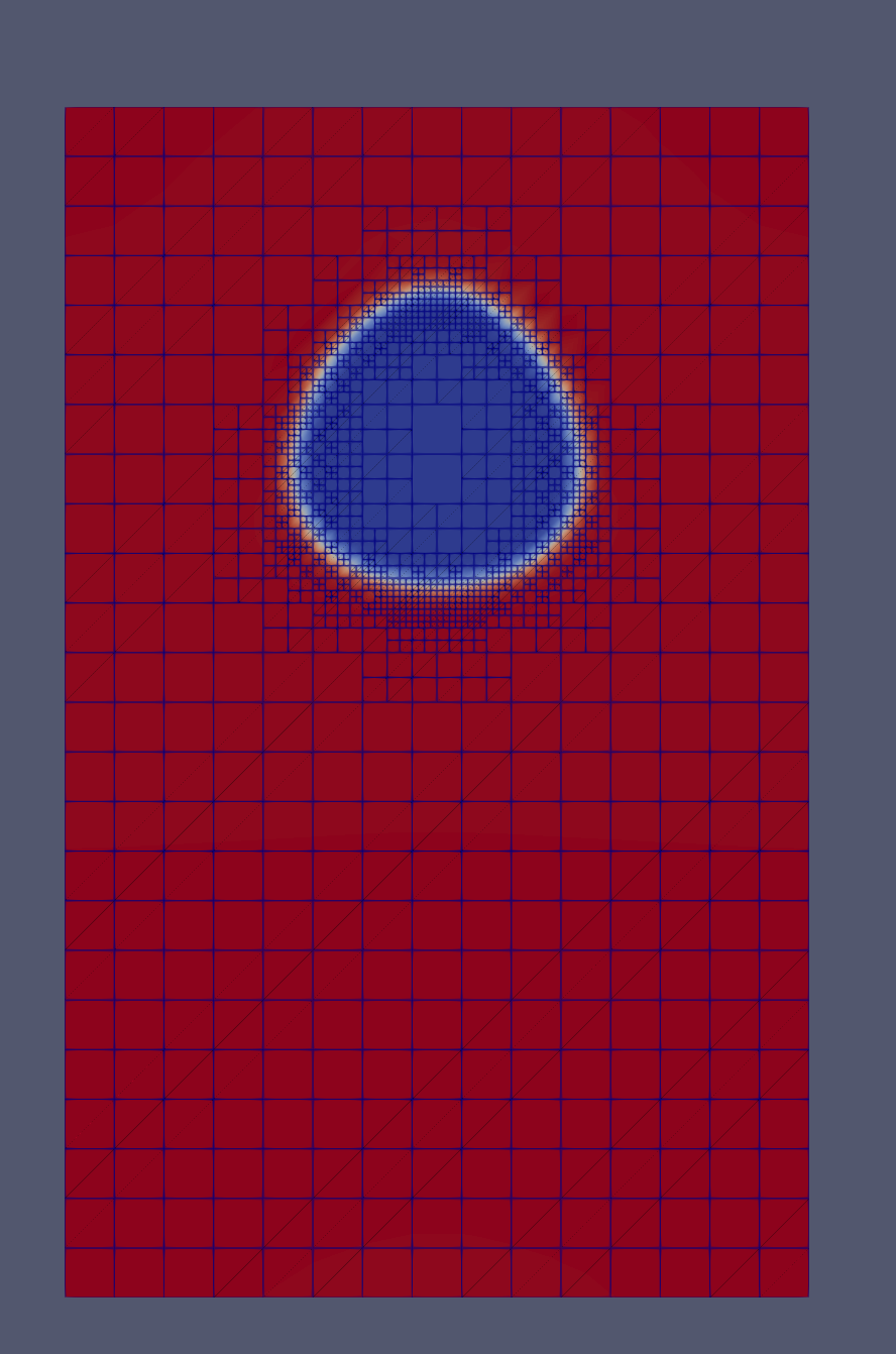
In the periodic configuration, the integral of $\phi$ is conserved. In the open configuration, it increases once the bubble leaves the domain through the top boundary, the bubble ($\phi=0$) being replaced by the matrix ($\phi=1$) entering at the bottom.

---

1. Clément Introïni. Interaction entre un fluide à haute température et un béton: contribution à la modélisation des échanges de masse et de chaleur. PhD thesis, Institut National Polytechnique de Toulouse-INPT, 2010. ↩