Example 3: time evolution of a polycristalline microstructures composed of 30 and 102 grains

Files

• 30 grains
  • Comprehensive test file (2D): main.cpp
  • Comprehensive test file (3D): main.cpp
  • 2D Reference results for comparison (regression test) (N=32, t=0.2): time_specialized.csv
  • 2D Reference results for comparison (N=128, t=25): time_specialized.csv
  • 3D Reference results for comparison (N=128, t=25): time_specialized.csv
• 102 grains
  • Comprehensive test file (2D): main.cpp
  • 2D Reference results for comparison (N=128, t=25): time_specialized.csv

Statement of the problem

This test extends to 30 and 102 grains the one presented in ¹ concerning the time evolution of a polycrystalline microstructure.

Allen-Cahn equations are solved in a square $\Omega=[0,32]\times[0,32]$ using an implicit monolithic algorithm.

$$\begin{align} \frac{\partial \eta_i}{\partial t} &= -L_i \frac{\delta F}{\delta \eta_i}, \qquad i = 1,\ldots,C \end{align}$$

where the free energy density is defined by:

$$\begin{align} F &= \int_V \left[ \sum_{i=1}^{N} \left( -\frac{1}{2}\eta_i^2 + \frac{1}{4}\eta_i^4 \right) + \sum_{i=1}^{C} \sum_{\substack{j=1 \\ j \neq i}}^{C} (\eta_i^2 \eta_j^2) + \sum_{i=1}^{C} \frac{\kappa_i}{2} \left|\nabla \eta_i \right|^2 \right] \, dv \end{align}$$

Hereabove, $C$ corresponds to the number of grains.

Initial condition

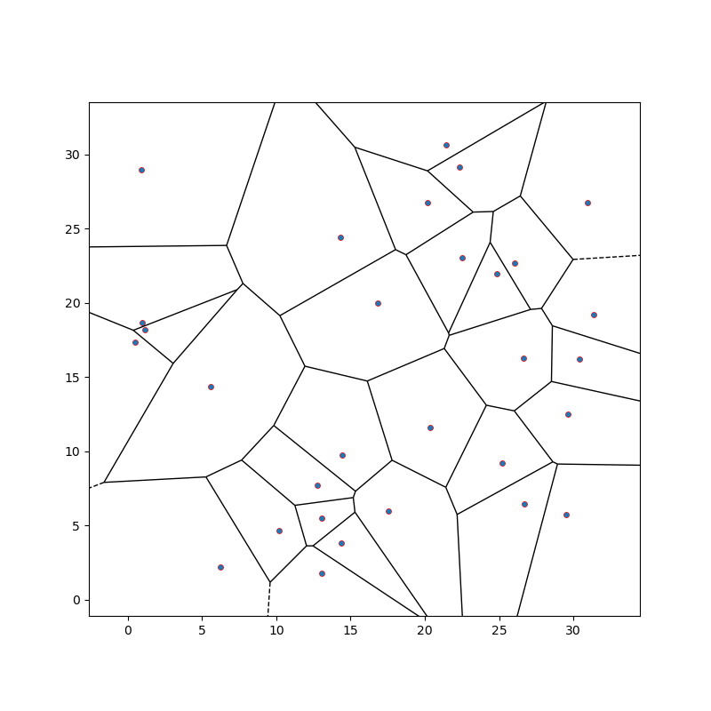
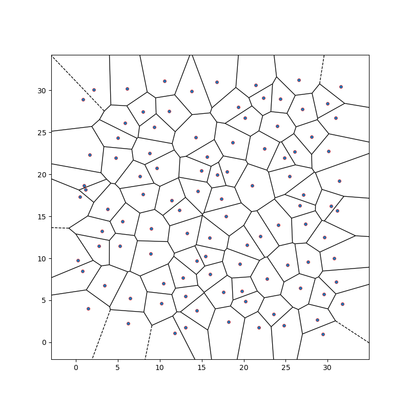
The Voronoi-based 2D initialization is generated using the Voro++ library.

Figure 1: initial polycrystalline microstructure composed of 30 grains.

Figure 2: initial polycrystalline microstructure composed of 102 grains.

Parameters used for the test

Description	Symbol	Value
mobility coefficients	$L_i$	$5.0$
energy gradient coefficients	$\kappa_i$	$0.1$

Boundary conditions

Periodic boundary conditions are prescribed on boundary of the domain.

Numerical scheme

• Time integration: Euler Implicit over the interval $t\in[0,25]$ with a time-step $\delta t=10^{-1}$.
• Spatial discretization for convergence analysis: uniform grid with $N={128}$ nodes in each spatial direction, with $\mathcal{Q}_1$ finite elements
• LBFGS solver: relative tolerance $10^{-10}$, absolute tolerance $10^{-14}$

Results

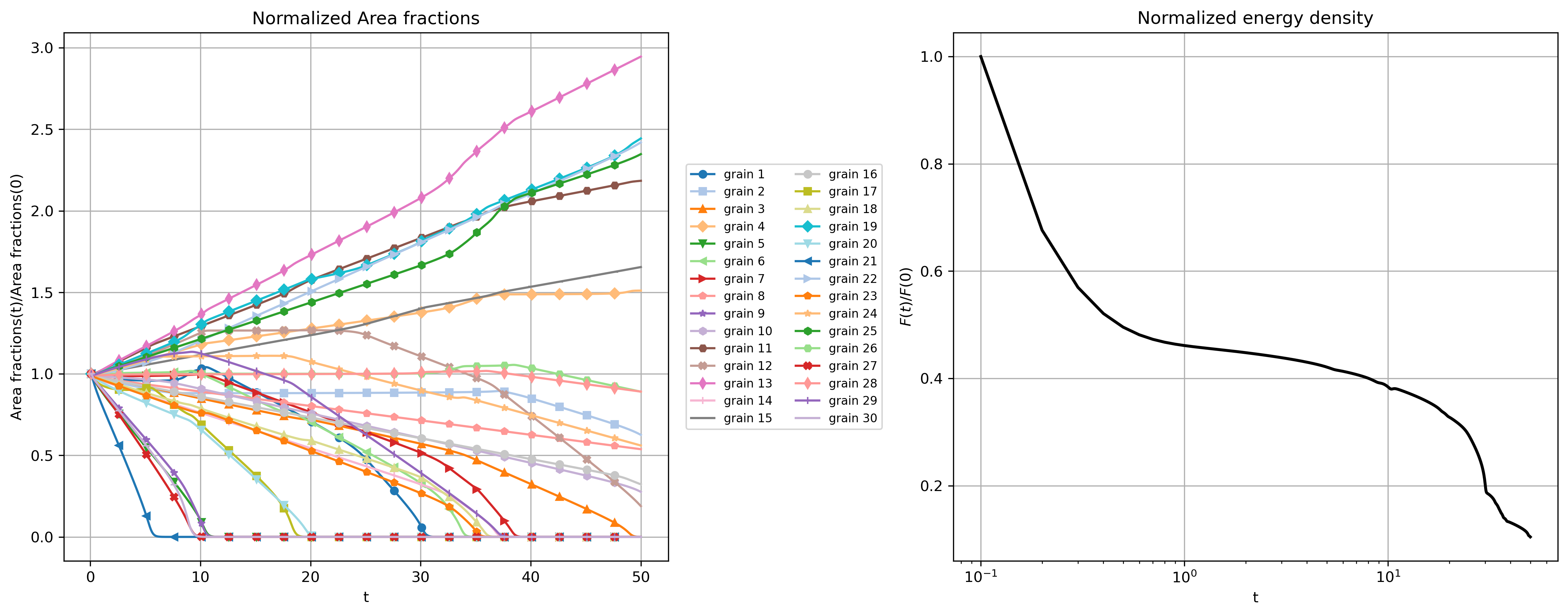
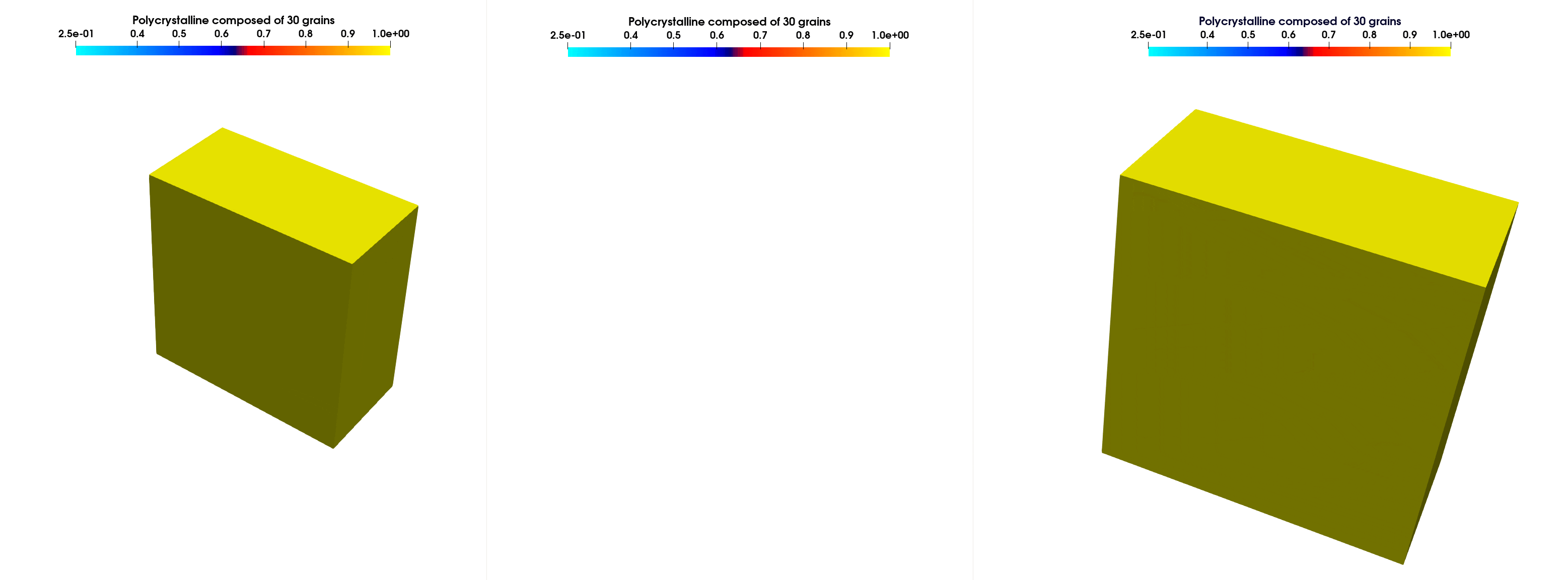
Figure 3 shows the time evolution of the normalized area and energy density for the polycrystalline microstructure composed of 30 grains. As shown on Figure 4, smaller grains tend to disappear, while larger grains grow. Figure 5 shows a 3D extension of the time evolution of the polycrystalline microstructure composed of 30 grains.

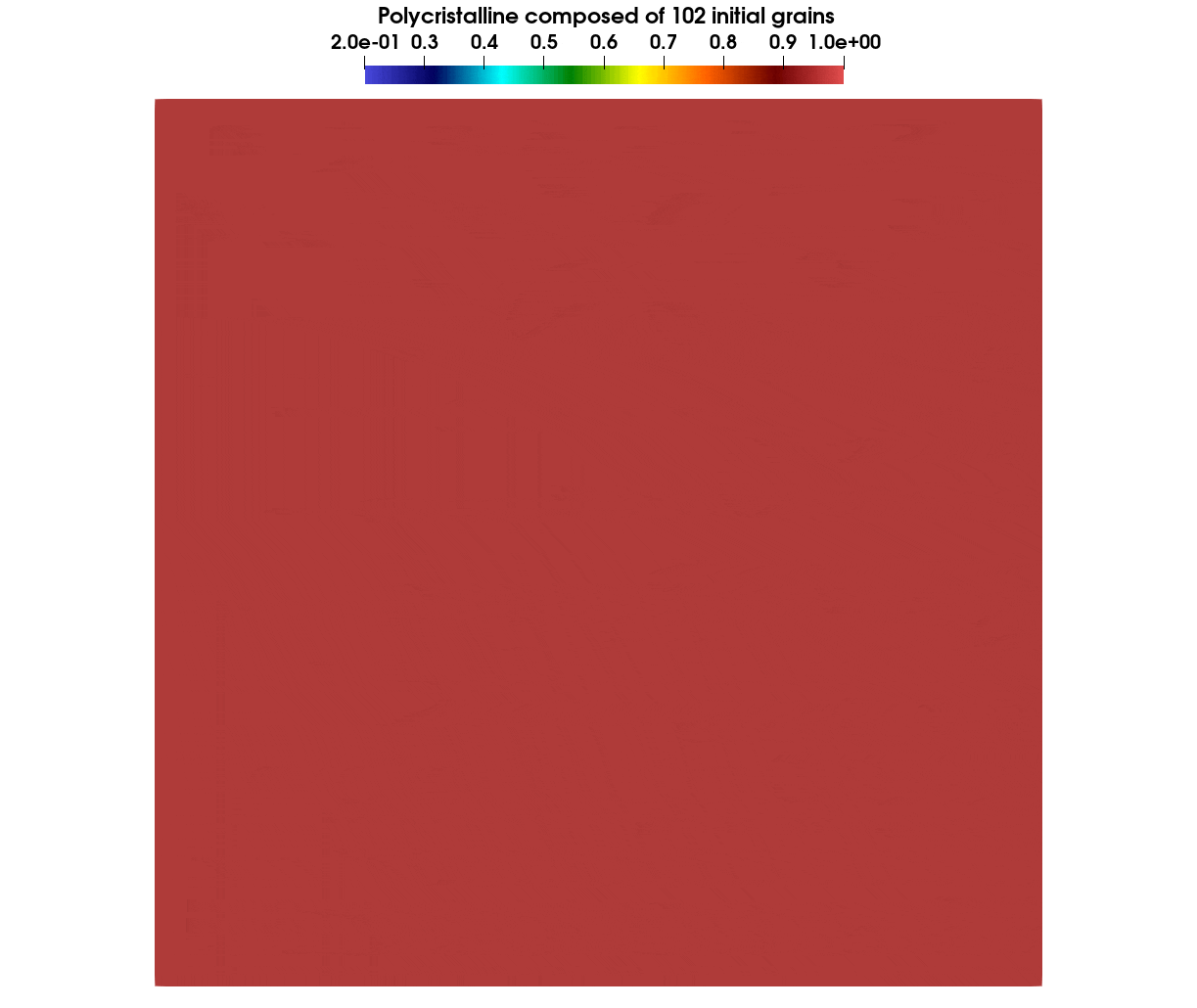
Figure 6 shows the time evolution of a polycrystalline microstructure composed of 102 grains.

Figure 3: normalized area and energy density

Figure 4: time evolution of the polycrystalline microstructure composed of 30 grains.

Figure 5: 3D extension of time evolution of the polycrystalline microstructure composed of 30 grains. (almost $2.10$ million DOF). The simulation has been performed with $2048$ MPI processes on Topaze supercomputer at CEA.

Figure 6: time evolution of the polycrystalline microstructure composed of 102 grains.

---

1. S Bulent Biner and others. Programming phase-field modeling. Springer, 2017. ↩