Example 3: spinodal decomposition

Files

• Comprehensive test file: main.cpp
• Reference results for comparison: time_specialized.csv

Statement of the problem

This test corresponds to the 2D simulation of spinodal decomposition proposed on PFhub

The domain $\Omega$ is a square $[0,200]\times[0,200]$

$$\begin{align} \frac{\partial \phi}{\partial t}&= M\Delta \mu \text{ in }\Omega \\[6pt] \mu &= F'(\phi) - \lambda \Delta \phi \text{ in }\Omega \end{align}$$

where $\phi$ is the phase indicator, $\mu$ the generalized chemical potential and $F'$ the derivative against $\phi$ of the potential $F$ defined by:

$$\begin{align} F(\phi)&=\omega(\phi - 0.3)^2 (0.7 - \phi)^2. \end{align}$$

Initial condition

The initial condition is defined by:

$$\phi = 0.5 + 0.01 \left[\cos(0.105x)\cos(0.11y) +(\cos(0.13x)\cos(0.087y))^2+ \cos(0.025x - 0.15y)\cos(0.07x - 0.02y)\right]$$

Figure 1: initial state

Parameters used for the test

For this test, the following parameters are considered:

Name	Description	Symbol	Value
mob	mobility coefficient	$M_\phi$	$5.0$
lambda	energy gradient coefficient	$\lambda$	$2.0$
omega	depth of the double-well potential	$\omega$	$5.0$

Boundary conditions

Neumann boundary conditions are prescribed on the boundary of the domain:

$$\begin{align} {\bf{n}} \cdot{} \lambda \nabla \phi&=0 \text{ on }\partial\Omega \\[6pt] {\bf{n}} \cdot{} \lambda \nabla \mu&=0 \text{ on }\partial\Omega \end{align}$$

Numerical scheme

• Time integration: Euler Implicit over the interval $t\in[0,10]$ (it could be extended further) with a time-step $\delta t=1$
• Spatial discretization: uniform grid with $N=100$ nodes in each spatial direction
• Newton solver: relative tolerance $10^{-12}$, absolute tolerance $10^{-12}$
• Iterative solver: HYPRE_GMRES
• Preconditioner: HYPRE_ILU

Results

The average value of $\phi$ is an available ouput of the simulation (see the file time_specialized.csv). It is defined by:

$$\dfrac{1}{|\Omega|}\displaystyle\int_{\Omega} \phi dv$$

For this test, the computed average value should remain constant over time.

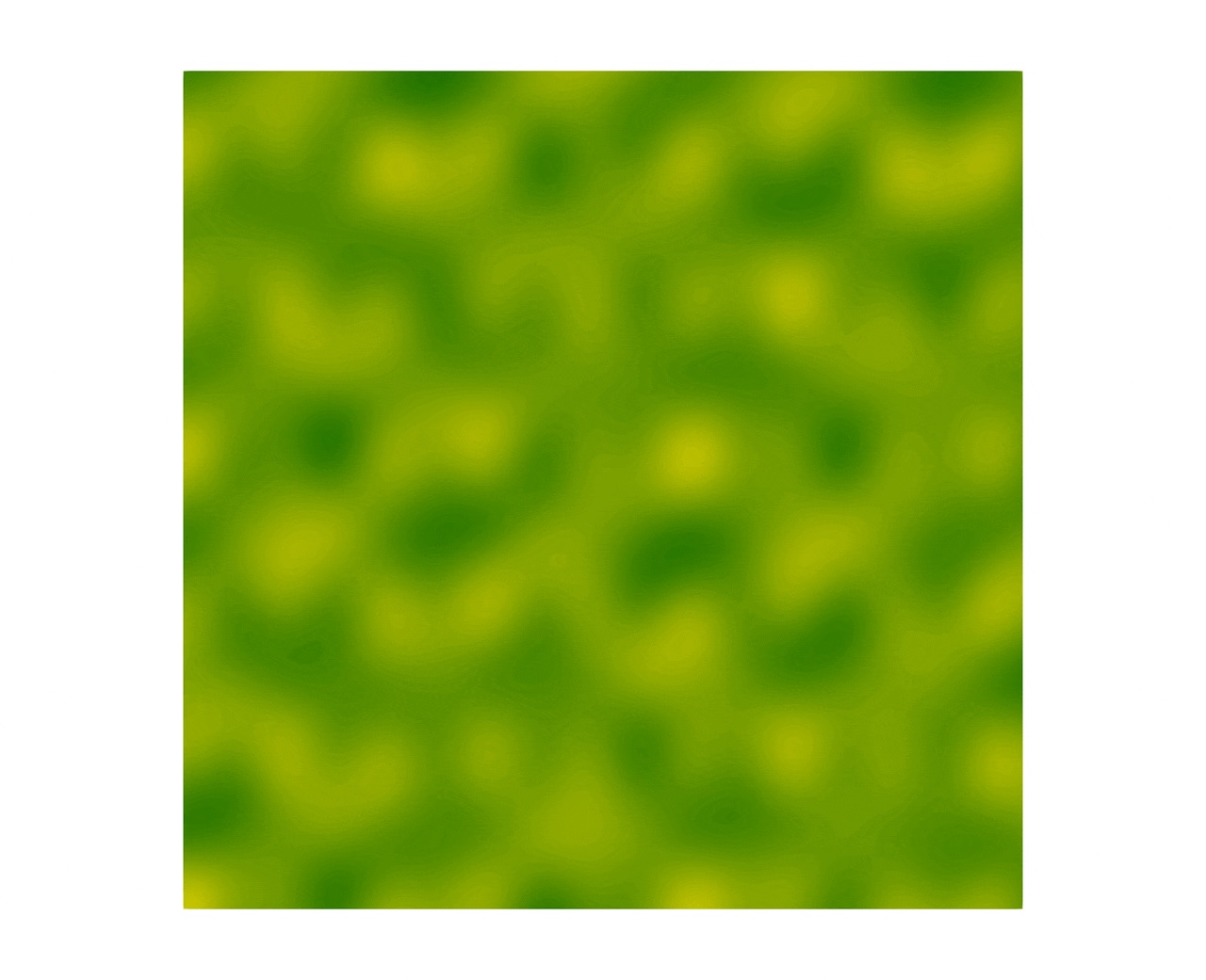
The figure 2 shows the spinodal decomposition, with a final simulation time set to $10000$.

Figure 2 : spinodal decomposition

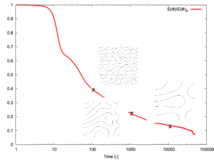
Figure 3 shows the time evolution of the normalized free-energy density, with snapshots taken at $100$, $1000$ and $10000$ s.

Figure 3 : time evolution of the normalized density of free energy