Example 4: steady-state solution of the Cahn–Hilliard equations

Files

• Comprehensive test file: main.cpp
• Reference results for comparison: convergence_output_ref.csv

Statement of the problem

This test consists of finding the steady-state solution of the Cahn–Hilliard equations. A transient simulation is performed to reach this steady-state, and a convergence analysis is carried out to ensure the consistency of the results.

The domain $\Omega$ is a square $[0,1]\times[0,1]$

$$\begin{align} \frac{\partial \phi}{\partial t}&=M \Delta \mu \text{ in }\Omega \\[6pt] \mu &= F'(\phi) - \lambda \Delta \phi \text{ in }\Omega \end{align}$$

where $\phi$ is the phase indicator, $\mu$ the generalized chemical potential and $F'$ the derivative against $\phi$ of the potential $F$ defined by:

$$\begin{align} F(\phi)&=\omega\phi^2(1-\phi)^2 \end{align}$$

Initial condition

The initial condition is given by:

$$\phi = \dfrac{1}{2} + \dfrac{1}{2} \tanh\left(\dfrac{x-0.5}{5\cdot 10^{-3}}\right).$$

Parameters used for the test

For this test, all parameters are equal to one.

Name	Description	Symbol	Value
mob	mobility coefficient	$M_\phi$	$1.0$
lambda	energy gradient coefficient	$\lambda$	$\dfrac{3}{2}{\sigma}{\epsilon}$
omega	depth of the double-well potential	$\omega$	$12\dfrac{\sigma}{\epsilon}$
sigma	surface tension	$\sigma$	$1.0$
epsilon	thickness of interface	$\epsilon$	$0.1$

Boundary conditions

Neumann boundary conditions are prescribed on boundary of the domain:

$$\begin{align} {\bf{n}} \cdot{} \lambda \nabla \phi&=0 \text{ on }\partial\Omega \\[6pt] {\bf{n}} \cdot{} \lambda \nabla \mu&=0 \text{ on }\partial\Omega \end{align}$$

Numerical scheme

• Time integration: Euler Implicit over the interval $t\in[0,1]$ with a time-step $\delta t=10^{-3}$. The calculation stops when convergence criteria are reached.

$$\|{\phi(t+\delta t)-\phi(t)}\|<\epsilon_\phi \\[6pt] \|{\mu(t+\delta t)-\mu(t)}\|<\epsilon_\mu$$

where $\epsilon_\phi=10^{-12}$ and $\epsilon_\mu=10^{-7}$.

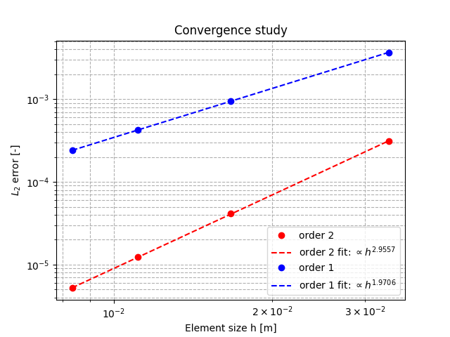
• Spatial discretization for convergence analysis: uniform grid with $N={30, 60, 90, 120}$ nodes in each spatial direction, with $\mathcal{Q}_1$ and $\mathcal{Q}_2$ finite elements
• Newton solver: relative tolerance $10^{-12}$, absolute tolerance $10^{-12}$
• Iterative solver: HYPRE_GMRES
• Preconditioner: HYPRE_ILU

Results

The steady state solution is given by:

$$\phi = \dfrac{1}{2} + \dfrac{1}{2} \tanh\left(\dfrac{x-0.5}{\epsilon}\right).$$

Figures 1 shows the results of convergence analysis with $\mathcal{Q}_1$ and $\mathcal{Q}_2$.

Figure 1: convergence analysis with $\mathcal{Q}_1$ and $\mathcal{Q}_2$ finite elements