Example 5: MMS benchmark

Files

• Comprehensive test file: main.cpp
• Reference results for comparison: convergence_output_ref.csv

Statement of the problem

This test is taken from Zhang & al.¹. It consists of spatial convergence analysis based on a manufactured solution benchmark.

The domain $\Omega$ is a square $[0,1]\times[0,1]$

$$\begin{align} \frac{\partial \phi}{\partial t}&= \Delta \mu +S(x,y,t)\text{ in }\Omega \\[6pt] \mu &= F'(\phi) - \lambda \Delta \phi \text{ in }\Omega \end{align}$$

where $\phi$ is the phase indicator, $\mu$ the generalized chemical potential and $F'$ the derivative against $\phi$ of the potential $F$ defined by:

$$\begin{align} F(\phi)&=\frac{\phi^4}{4} - \frac{\phi^2}{2} \end{align}$$

In equation (1), $S(x,y,t)$ is the source term allowing the exact solution:

$$\phi = (t+1) \sin(\alpha \pi x)$$

Initial condition

The initial condition is given by:

$$\phi = \sin(\alpha \pi x)$$

For this test, $\alpha$ is set to $1$.

Parameters used for the test

For this test, all parameters are equal to one.

Name	Description	Symbol	Value
mob	mobility coefficient	$M_\phi$	$1.0$
lambda	energy gradient coefficient	$\lambda$	$1.0$
omega	depth of the double-well potential	$\omega$	$1.0$

Boundary conditions

Neumann boundary conditions are prescribed on the top and bottom of the domain:

$$\begin{align} {\bf{n}} \cdot{} \lambda \nabla \phi&=0 \text{ on }\partial\Omega_{top}\cup\partial\Omega_{bottom} \\[6pt] {\bf{n}} \cdot{} \lambda \nabla \mu&=0 \text{ on }\partial\Omega_{top}\cup\partial\Omega_{bottom} \end{align}$$

Dirichlet boundary conditions are prescribed on the right and left of the domain:

$$\begin{align} \phi&=0 \text{ on }\partial\Omega_{left}\cup\partial\Omega_{right} \\[6pt] \mu&=0 \text{ on }\partial\Omega_{left}\cup\partial\Omega_{right} \end{align}$$

Numerical scheme

• Time integration: Euler Implicit over the interval $t\in[0,1]$ with a time-step $\delta t=1$.
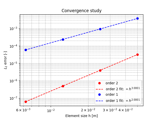
• Spatial discretization for convergence analysis: uniform grid with $N={160, 80, 40, 20}$ nodes in each spatial direction, with $\mathcal{Q}_1$ and $\mathcal{Q}_2$ finite elements
• Newton solver: relative tolerance $10^{-8}$, absolute tolerance $10^{-12}$
• Iterative solver: HYPRE_GMRES
• Preconditioner: HYPRE_ILU

Results

Figures 1 shows the results of convergence analysis with $\mathcal{Q}_1$ and $\mathcal{Q}_2$.

Figure 1: convergence analysis with $\mathcal{Q}_1$ and $\mathcal{Q}_2$ finite elements

---

1. Liangzhe Zhang, Michael R Tonks, Derek Gaston, John W Peterson, David Andrs, Paul C Millett, and Bulent S Biner. A quantitative comparison between c0 and c1 elements for solving the cahn–hilliard equation. Journal of Computational Physics, 236:74–80, 2013. ↩