Example 2: sintering of nine unequal sized particles Files Statement of the problem This test is a Finite Element version of the sintering test of nine unequal sized particles from
Allen-Cahn (AC) and Cahn-Hilliard (CH) equations are solved in a square Ω = [ 0 , 50 ] × [ 0 , 50 ] \Omega=[0,50]\times[0,50] Ω = [ 0 , 50 ] × [ 0 , 50 ]
( C H ) ∂ ρ ∂ t = ∇ ⋅ D ∇ ( ∂ f ∂ ρ − κ ρ ∇ 2 ρ ) ( A C ) ∂ η i ∂ t = − L ( ∂ f ∂ η i − κ η ∇ 2 η i ) , i = 1 , 9
\begin{align}
(CH)\quad \frac{\partial \rho}{\partial t}
&=
\nabla \cdot
D \nabla
\left(
\frac{\partial f}{\partial \rho}
-
\kappa_{\rho}\nabla^{2}\rho
\right)
\\[5pt]
(AC)\quad \frac{\partial \eta_i}{\partial t}
&=
-L\left(
\frac{\partial f}{\partial \eta_i}
-
\kappa_{\eta}\nabla^{2}\eta_i
\right), \quad i=1,9
\end{align}
( C H ) ∂ t ∂ ρ ( A C ) ∂ t ∂ η i = ∇ ⋅ D ∇ ( ∂ ρ ∂ f − κ ρ ∇ 2 ρ ) = − L ( ∂ η i ∂ f − κ η ∇ 2 η i ) , i = 1 , 9
The mobility coefficient D D D
D = D v o l p ( ρ ) + D v a p [ 1 − p ( ρ ) ] + D s u r f ρ ( 1 − ρ ) + D g b ∑ i ∑ i ≠ m η i η m p ( ρ ) = ρ 3 ( 6 ρ 2 − 15 ρ + 10 )
\begin{align}
D
&=
D_{\mathrm{vol}}p(\rho)
+
D_{\mathrm{vap}}\left[1-p(\rho)\right]
+
D_{\mathrm{surf}}\rho(1-\rho)
+
D_{\mathrm{gb}}
\sum_i \sum_{i\neq m}\eta_i\eta_m
\\[5pt]
p(\rho)&=\rho^3(6\rho^2-15\rho +10)
\end{align}
D p ( ρ ) = D vol p ( ρ ) + D vap [ 1 − p ( ρ ) ] + D surf ρ ( 1 − ρ ) + D gb i ∑ i = m ∑ η i η m = ρ 3 ( 6 ρ 2 − 15 ρ + 10 )
The free energy density is defined by:
F = ∫ V [ f ( ρ , η 1 … p ) + κ ρ 2 ( ∇ ρ ) 2 + ∑ i κ η 2 ( ∇ η i ) 2 ] d v
\begin{align}
F
&=
\int_V
\left[
f(\rho,\eta_{1\ldots p})
+
\frac{\kappa_{\rho}}{2}(\nabla \rho)^2
+
\sum_i
\frac{\kappa_{\eta}}{2}
(\nabla \eta_i)^2
\right]
\, dv
\end{align}
F = ∫ V [ f ( ρ , η 1 … p ) + 2 κ ρ ( ∇ ρ ) 2 + i ∑ 2 κ η ( ∇ η i ) 2 ] d v
where
f ( ρ , η i … p ) = 16 ρ 2 ( 1 − ρ ) 2 + [ ρ 2 + 6 ( 1 − ρ ) ∑ i η i 2 − 4 ( 2 − ρ ) ∑ i η i 3 + 3 ( ∑ i η i 2 ) 2 ]
\begin{align}
f(\rho,\eta_{i\ldots p})
&=
16\rho^{2}(1-\rho)^{2}
+
\left[
\rho^{2}
+
6(1-\rho)\sum_i \eta_i^{2}
-
4(2-\rho)\sum_i \eta_i^{3}
+
3\left(\sum_i \eta_i^{2}\right)^{2}
\right]
\end{align}
f ( ρ , η i … p ) = 16 ρ 2 ( 1 − ρ ) 2 + ⎣ ⎡ ρ 2 + 6 ( 1 − ρ ) i ∑ η i 2 − 4 ( 2 − ρ ) i ∑ η i 3 + 3 ( i ∑ η i 2 ) 2 ⎦ ⎤
Initial condition The initial condition for the Cahn-Hilliard equation is given by:
ρ ( x , 0 ) = { 1 , ( x − 14.5 ) 2 + ( y − 25 ) 2 < 5 , 1 , ( x − 35.5 ) 2 + ( y − 25 ) 2 < 5 , 1 , ( x − 25 ) 2 + ( y − 14.5 ) 2 < 5 1 , ( x − 25 ) 2 + ( y − 35.5 ) 2 < 5 , 1 , ( x − 25 ) 2 + ( y − 25 ) 2 < 5 , 1 , ( x − 19.5 ) 2 + ( y − 19.5 ) 2 < 2.5 , 1 , ( x − 30.5 ) 2 + ( y − 19.5 ) 2 < 2.5 1 , ( x − 19.5 ) 2 + ( y − 30.5 ) 2 < 2.5 , 1 , ( x − 30.5 ) 2 + ( y − 30.5 ) 2 < 2.5 , 0 , otherwise .
\begin{align}
\rho(\mathbf{x}, 0) &=
\begin{cases}
1, & \sqrt{(x - 14.5)^2 + (y - 25)^2} < 5, \\
1, & \sqrt{(x - 35.5)^2 + (y - 25)^2} < 5, \\
1, & \sqrt{(x - 25)^2 + (y - 14.5)^2} < 5 \\
1, & \sqrt{(x - 25)^2 + (y - 35.5)^2} < 5, \\
1, & \sqrt{(x - 25)^2 + (y - 25)^2} < 5, \\
1, & \sqrt{(x - 19.5)^2 + (y - 19.5)^2} < 2.5, \\
1, & \sqrt{(x - 30.5)^2 + (y - 19.5)^2} < 2.5 \\
1, & \sqrt{(x - 19.5)^2 + (y - 30.5)^2} < 2.5, \\
1, & \sqrt{(x - 30.5)^2 + (y - 30.5)^2} < 2.5, \\
0, & \text{otherwise}.
\end{cases}
\end{align}
ρ ( x , 0 ) = ⎩ ⎨ ⎧ 1 , 1 , 1 , 1 , 1 , 1 , 1 , 1 , 1 , 0 , ( x − 14.5 ) 2 + ( y − 25 ) 2 < 5 , ( x − 35.5 ) 2 + ( y − 25 ) 2 < 5 , ( x − 25 ) 2 + ( y − 14.5 ) 2 < 5 ( x − 25 ) 2 + ( y − 35.5 ) 2 < 5 , ( x − 25 ) 2 + ( y − 25 ) 2 < 5 , ( x − 19.5 ) 2 + ( y − 19.5 ) 2 < 2.5 , ( x − 30.5 ) 2 + ( y − 19.5 ) 2 < 2.5 ( x − 19.5 ) 2 + ( y − 30.5 ) 2 < 2.5 , ( x − 30.5 ) 2 + ( y − 30.5 ) 2 < 2.5 , otherwise .
The initial conditions for the Allen-Cahn equations are given by:
η 1 ( x , 0 ) = { 1 ( x − 14.5 ) 2 + ( y − 25 ) 2 < 5 , 0 otherwise .
\begin{align}
\eta_1(\mathbf{x}, 0) &=
\begin{cases}
1 & \sqrt{(x - 14.5)^2 + (y - 25)^2} < 5, \\
0 & \text{otherwise}.
\end{cases}
\end{align}
η 1 ( x , 0 ) = { 1 0 ( x − 14.5 ) 2 + ( y − 25 ) 2 < 5 , otherwise .
η 2 ( x , 0 ) = { 1 ( x − 35.5 ) 2 + ( y − 25 ) 2 < 5 , 0 otherwise .
\begin{align}
\eta_2(\mathbf{x}, 0) &=
\begin{cases}
1 & \sqrt{(x - 35.5)^2 + (y - 25)^2} < 5, \\
0 & \text{otherwise}.
\end{cases}
\end{align}
η 2 ( x , 0 ) = { 1 0 ( x − 35.5 ) 2 + ( y − 25 ) 2 < 5 , otherwise .
η 3 ( x , 0 ) = { 1 ( x − 25 ) 2 + ( y − 14.5 ) 2 < 5 , 0 otherwise .
\begin{align}
\eta_3(\mathbf{x}, 0) &=
\begin{cases}
1 & \sqrt{(x - 25)^2 + (y - 14.5)^2} < 5, \\
0 & \text{otherwise}.
\end{cases}
\end{align}
η 3 ( x , 0 ) = { 1 0 ( x − 25 ) 2 + ( y − 14.5 ) 2 < 5 , otherwise .
η 4 ( x , 0 ) = { 1 , ( x − 25 ) 2 + ( y − 35.5 ) 2 < 5 , 0 , otherwise .
\begin{align}
\eta_4(\mathbf{x}, 0) &=
\begin{cases}
1, & \sqrt{(x - 25)^2 + (y - 35.5)^2} < 5, \\
0, & \text{otherwise}.
\end{cases}
\end{align}
η 4 ( x , 0 ) = { 1 , 0 , ( x − 25 ) 2 + ( y − 35.5 ) 2 < 5 , otherwise .
η 5 ( x , 0 ) = { 1 , ( x − 25 ) 2 + ( y − 25 ) 2 < 5 , 0 , otherwise .
\begin{align}
\eta_5(\mathbf{x}, 0) &=
\begin{cases}
1, & \sqrt{(x - 25)^2 + (y - 25)^2} < 5, \\
0, & \text{otherwise}.
\end{cases}
\end{align}
η 5 ( x , 0 ) = { 1 , 0 , ( x − 25 ) 2 + ( y − 25 ) 2 < 5 , otherwise .
η 6 ( x , 0 ) = { 1 , ( x − 19.5 ) 2 + ( y − 19.5 ) 2 < 2.5 , 0 , otherwise .
\begin{align}
\eta_6(\mathbf{x}, 0) &=
\begin{cases}
1, & \sqrt{(x - 19.5)^2 + (y - 19.5)^2} < 2.5, \\
0, & \text{otherwise}.
\end{cases}
\end{align}
η 6 ( x , 0 ) = { 1 , 0 , ( x − 19.5 ) 2 + ( y − 19.5 ) 2 < 2.5 , otherwise .
η 7 ( x , 0 ) = { 1 , ( x − 30.5 ) 2 + ( y − 19.5 ) 2 < 2.5 , 0 , otherwise .
\begin{align}
\eta_7(\mathbf{x}, 0) &=
\begin{cases}
1, & \sqrt{(x - 30.5)^2 + (y - 19.5)^2} < 2.5, \\
0, & \text{otherwise}.
\end{cases}
\end{align}
η 7 ( x , 0 ) = { 1 , 0 , ( x − 30.5 ) 2 + ( y − 19.5 ) 2 < 2.5 , otherwise .
η 8 ( x , 0 ) = { 1 , ( x − 19.5 ) 2 + ( y − 30.5 ) 2 < 2.5 , 0 , otherwise .
\begin{align}
\eta_8(\mathbf{x}, 0) &=
\begin{cases}
1, & \sqrt{(x - 19.5)^2 + (y - 30.5)^2} < 2.5, \\
0, & \text{otherwise}.
\end{cases}
\end{align}
η 8 ( x , 0 ) = { 1 , 0 , ( x − 19.5 ) 2 + ( y − 30.5 ) 2 < 2.5 , otherwise .
η 9 ( x , 0 ) = { 1 , ( x − 30.5 ) 2 + ( y − 30.5 ) 2 < 2.5 , 0 , otherwise .
\begin{align}
\eta_9(\mathbf{x}, 0) &=
\begin{cases}
1, & \sqrt{(x - 30.5)^2 + (y - 30.5)^2} < 2.5, \\
0, & \text{otherwise}.
\end{cases}
\end{align}
η 9 ( x , 0 ) = { 1 , 0 , ( x − 30.5 ) 2 + ( y − 30.5 ) 2 < 2.5 , otherwise .
Parameters used for the test
Description
Symbol
Value
mobility coefficient (AC)
L L L 10.0 10.0 10.0
energy gradient coefficient (AC)
κ η \kappa_\eta κ η 5 5 5
energy gradient coefficient (CH)
κ ρ \kappa_\rho κ ρ 2 2 2
bulk diffusivity in the lattice (CH)
D v o l D_{\mathrm{vol}} D vol 0.04 0.04 0.04
diffusivity of the vapor phase (CH)
D v a p D_{\mathrm{vap}} D vap 0.002 0.002 0.002
surface diffusivity (CH)
D s u r f D_{\mathrm{surf}} D surf 16 16 16
grain boundary diffusivity (CH)
D g b D_{\mathrm{gb}} D gb 1.6 1.6 1.6
Boundary conditions Neumann boundary conditions are prescribed on boundary of the domain.
Numerical scheme
Time integration: Euler Implicit over the interval t ∈ [ 0 , 0.25 ] t\in[0,0.25] t ∈ [ 0 , 0.25 ] δ t = 1 0 − 4 \delta t=10^{-4} δ t = 1 0 − 4
Spatial discretization for convergence analysis: uniform grid with N = 200 N={200} N = 200 Q 1 \mathcal{Q}_1 Q 1
Newton solver: relative tolerance 1 0 − 10 10^{-10} 1 0 − 10 1 0 − 14 10^{-14} 1 0 − 14
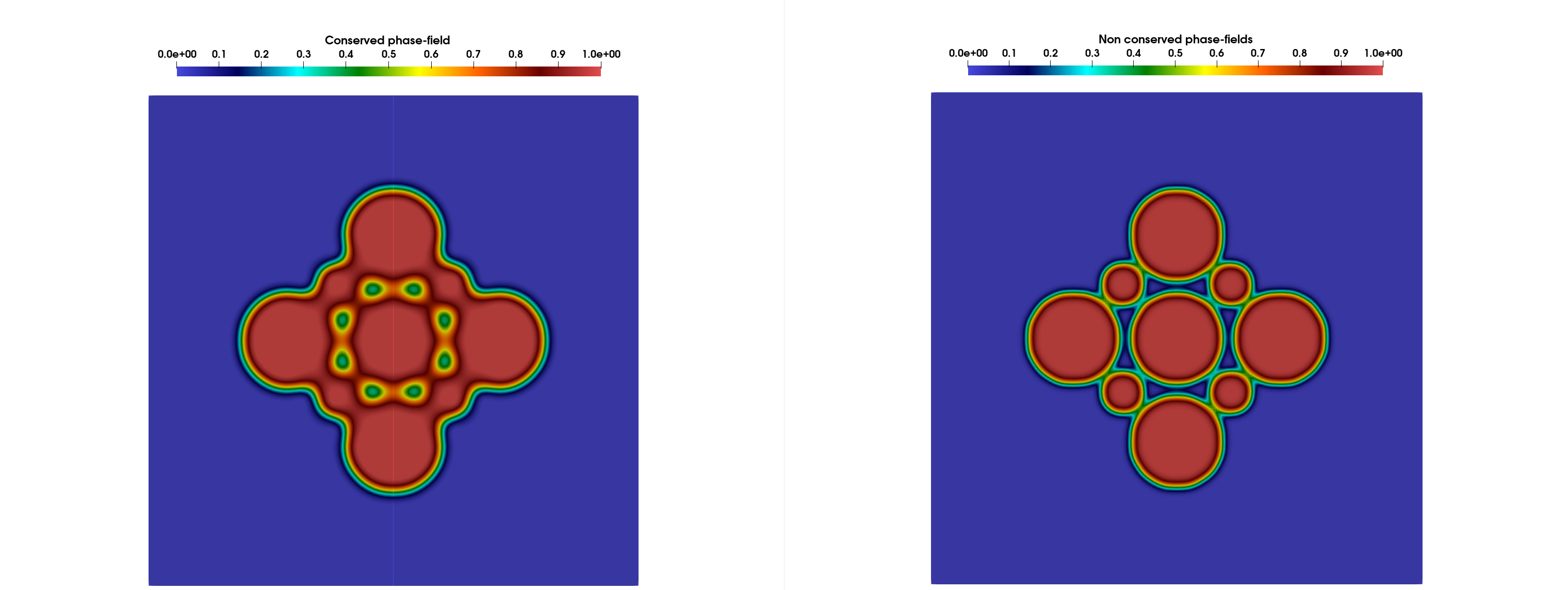
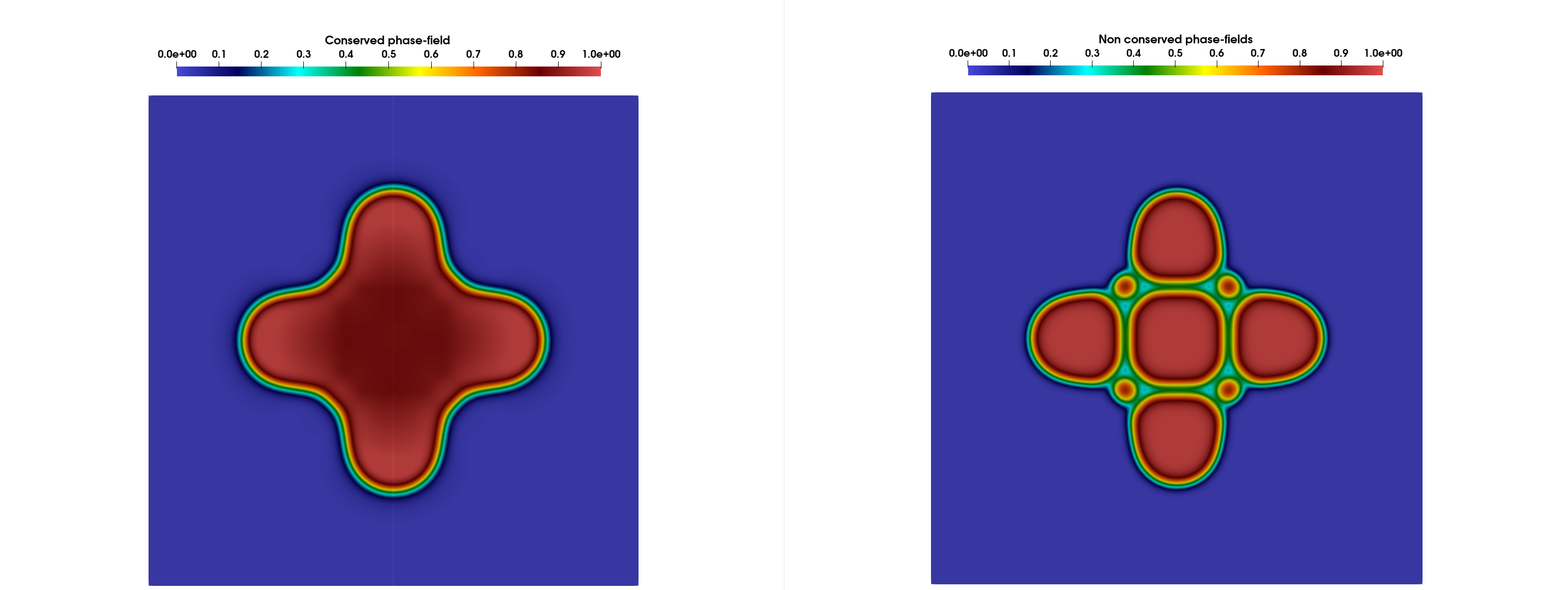
Results Figure 1 shows the evolution of conserved and non conserved phase-fields at time step 100 and 2500 (from top to bottom).
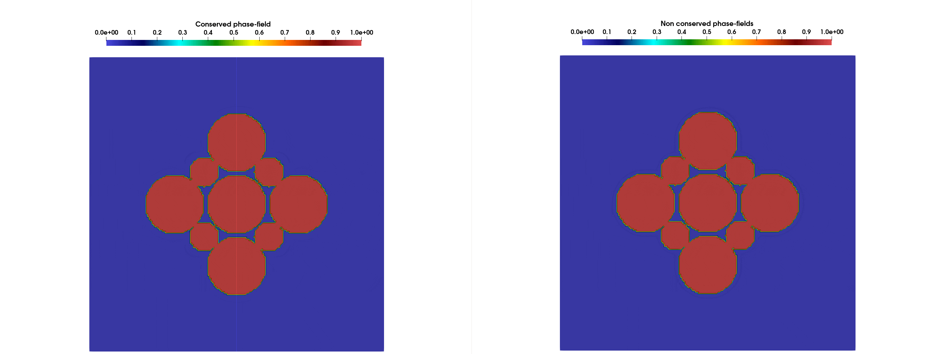
Figure 2 shows the time evolution of nine unequal sized particles.
The results are in good agreement with those presented in
Figure 1: evolution of conserved and non conserved phase-fields at time step 100 and 2500 (from top to bottom).
Figure 2: time evolution of nine unequal sized particles.
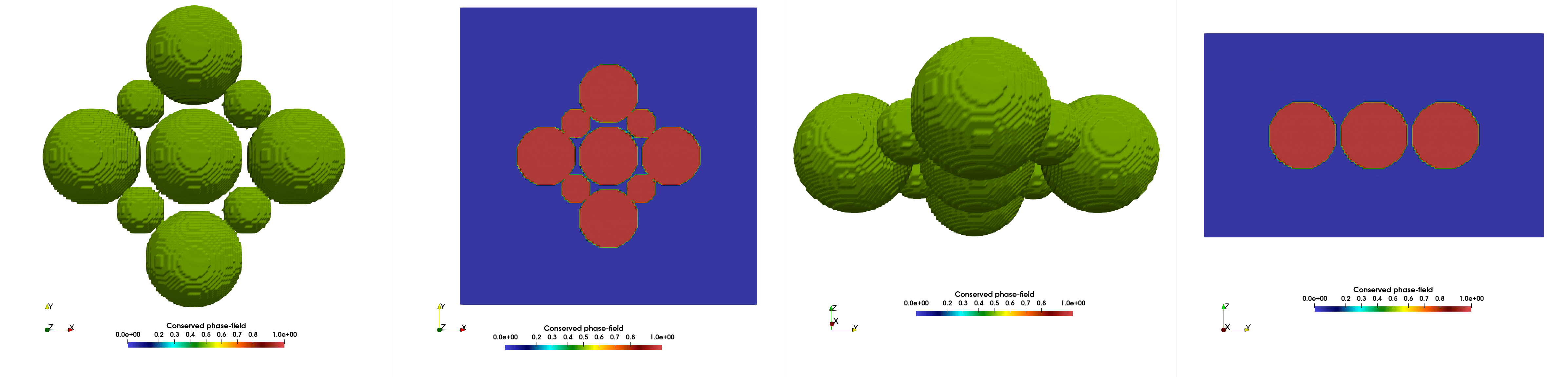
Figure 3: 3D extension of the time evolution of nine unequal sized particles (4.8 4.8 4.8 4096 4096 4096